Dijkstras Algorithm Visualizer

Dijkstra’s algorithm is (in my opinion) one of the most interesting algorithms created, because of its simplicity, history, complexity, and extensibility.

This project utilized mathematical computing technologies such as Matplotlib and Networkx to iteratively create a visualization for dijkstra’s algorithm.

Terminology: Graphs are collections of nodes and edges, where nodes are “points” and edges are “connections” between different nodes. Graphs have a million and a half different uses in computer science because they are so versatile. They exist to model relations between discrete objects. Within the context of this write-up, a network is used interchangeably with the idea of a graph. This is not entirely correct, although computer networks can be modeled using graphs, where each node is a computer terminal and each edge is a connection to other computers, modems, etc.

Examples

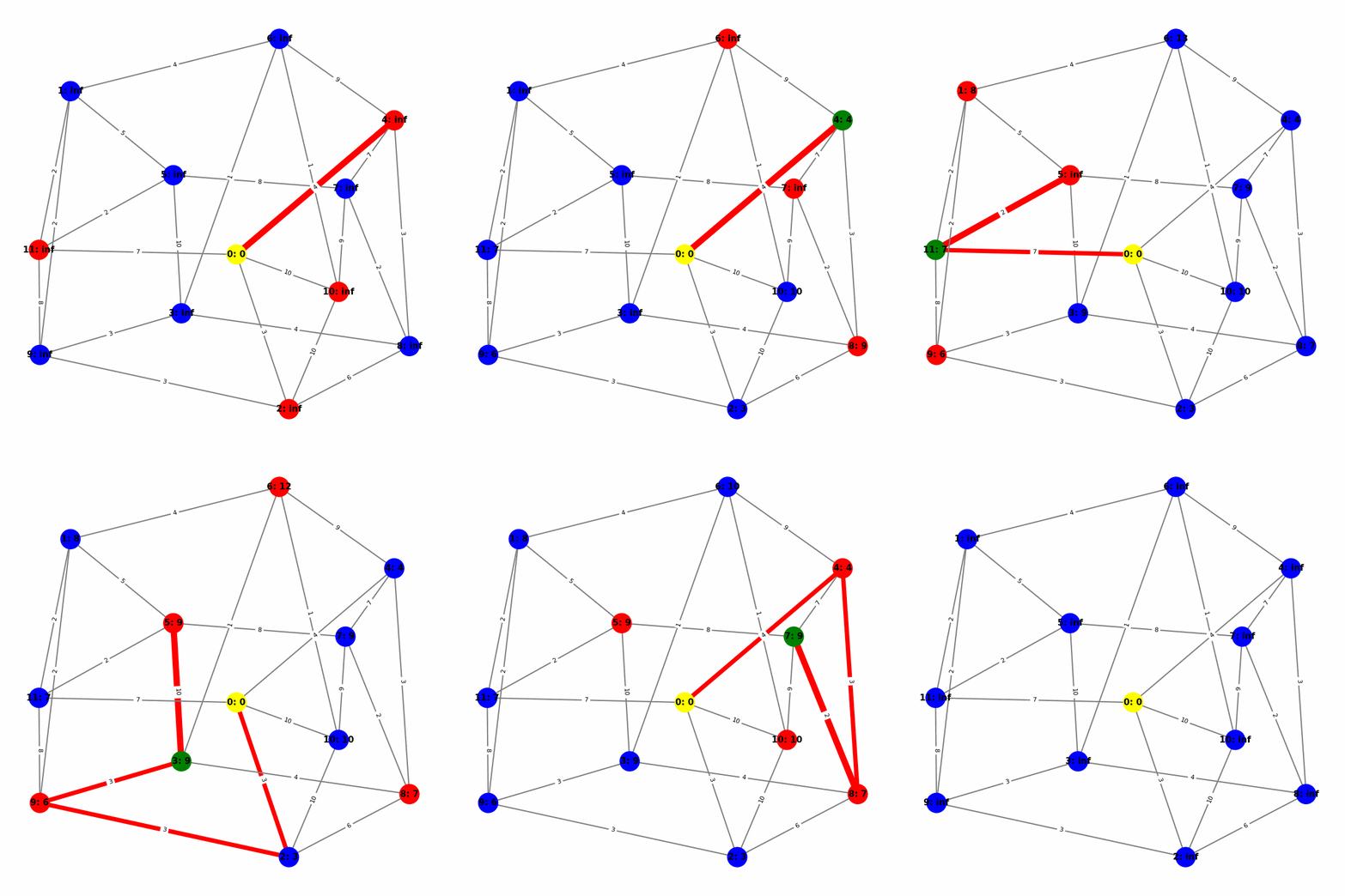
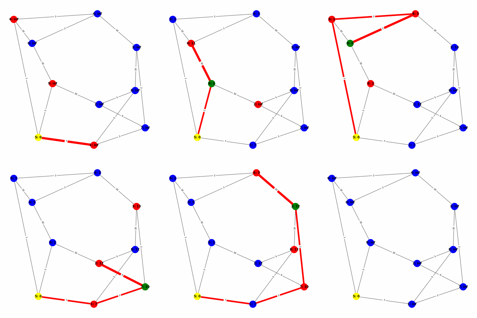
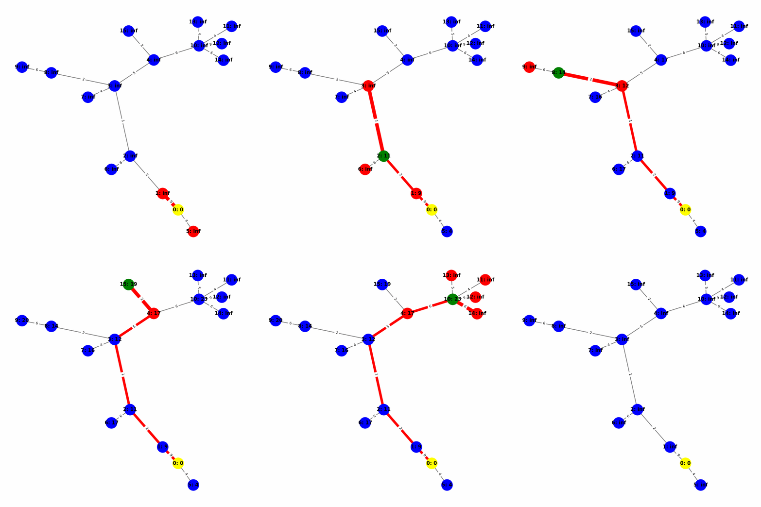
Here are a couple different graphs that can be visualized with this tool:

Understanding the Visuals

To understand the various visuals included above, lets take a look at the algorithmic portion of the project’s source code:

# dist will be a dictionary that stores the distances from every node to our start node
dist = {start_node:0}

# this is a dictionary of nodes that you work backwards from to construct the shortest path
# from any given node to the start node.
predecessor_dict = {start_node: start_node}
node_queue = [] # all the different nodes we have to visit

#start by setting all node distances except source to infinite.
for node in G.nodes:
    if node != start_node:
        dist[node] = float('inf')

    node_queue.append( (dist[node], node) ) #add tuple of (distance, node) to priority queue
        
while len(node_queue):  # while items in node_queue
    work_node = min(node_queue) # work off of the closest node
    node_queue.remove(work_node) #get and pop minimum of node_queue (using list as a min-priority here)
    work_node = work_node[1] #strip weight/distance that node name was packaged with

    # for every neighbor (shares an edge) with the work node
    for adj_node in G.adj[work_node]:
        # try constructing a path from current node to the neighbor node
        alt_path = dist[work_node] + G[work_node][adj_node]["weight"]

        # for each adjacent node to the work node, see if its path is shorter than prior believed distance   
        # first time around, dist[adj_node] is inf, so will always update
        # however, we always check because there could be shortcuts hidden within weighted edges       
        if alt_path < dist[adj_node]:

            # update proper distances and edges, change priority of adj_node 
            # (could be a shorter path now!)
            node_queue[node_queue.index((dist[adj_node], adj_node))] = (alt_path, adj_node) 
            dist[adj_node] = alt_path

            #  each node points to its predecessor in path, follow pointers
            #  until start node is reached to construct physical shortest path
            predecessor_dict[adj_node] = work_node  
            

You can find this within the whole_dijkstra() function, however it is bloated with animation code for the visualizer. Above I have trimmed out the non-essential steps of the algorithm.

• We start by choosing a node to use at the origin of Dijkstra’s algorithm.
• Also as part of the setup, we initialize every other node to have a distance of inf from our origin.
• Insert every node of the graph into an array/queue/datastructure of choice

getting to the good part…

Now, for every node in the queue:

• we select the closest node, and visit every neighbor to it
• check if the path to the working node and the neighbor is superior to a preexisting path to a neighbor
• update proper items. Within our example, we have a Dist map, where keys are nodes, and values are distances from origin. Additionally, I am using a predecessor map where each key is a node, and each value is the optimal node to ‘step’ backwards to to actually find what the shortest path to the origin is.

And that is it! We see this type of behaviour within the visualizer.

• Yellow node is the origin, with name:distance, where distiance is always trivially 0.
• Green node is the current working node, where we are visiting all of its neighbors, the Red nodes.
• Blue nodes are unvisited.
• The current edge is highlighted with thick red to show that is the connection the algorithm is currently investigating. The thin red edges are the optimal path back to the root.

Worth

Dijkstra’s algorithm shows up in many different problems. It is a simple way to find the shortest paths from one node in a graph (the origin) to every other node in the graph.